The process of clustering usually involves variable standardization. This post illustrates the effect of this important data pre-processing step on the result of k-means clustering with R using a small data set of groceries shopping.
Clustering, distances, k-means
Clustering refers to a very broad set of techniques for finding subgroups, or clusters, in a data set. When we cluster the observations of a data set, we seek to partition them into distinct groups so that
- the observations within each group are quite “similar” to each other,
- while observations in different groups are quite “different” from each other.
There are many possible ways to define the concept of “(dis)similarity,” but by far the most common choice involves squared Euclidean distance (James et al. 2017, 385–87).
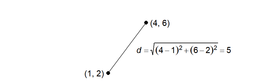
The Euclidean distance of two points \((x_1, y_1)\) and \((x_2,y_2)\) in a 2-dimensional space is calculated as
\[\sqrt{(x_2−x_1)^2+(y_2−y_1)^2}\text{.}\] For example, if we are given two points with coordinates (1, 2) and (4, 6) then the Euclidean distance \(d\) between these points is 5:
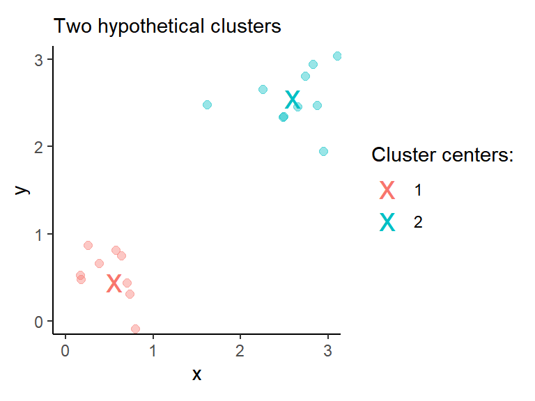
Let’s take k-means clustering. The algorithm aims to partition observations into k groups such that the sum of squared distances from observations to the assigned cluster centers is minimized. In the example plotted below, there are two distinct clusters (\(k=2\)) with 10 observations in each. Cluster centers are highlighted with colored crosses.
Surprise
Imagine you have a purchasing history of customers in a local shop. You would like to cluster them into groups with similar purchasing habits to target them later with different offers and marketing materials. For simplicity, you pick only four customers and their history of purchasing caviar and bread during the last month, both measured in kilograms. You aggregate data on a customer level and get the table below (available in csv here):
# Attach packages.
library(tidyverse)
# Import groceries data.
groceries_df <- read_delim(file = "groceries.csv", delim = ";")| Customer | Caviar (kg) | Bread (kg) |
|---|---|---|
| Artis | 0.0 | 10.0 |
| Baiba | 0.1 | 9.0 |
| Cintija | 1.0 | 7.5 |
| Dainis | 1.1 | 4.5 |
Below is the same data in the scatter plot. Please do a mental exercise and assign these four customers into two clusters.
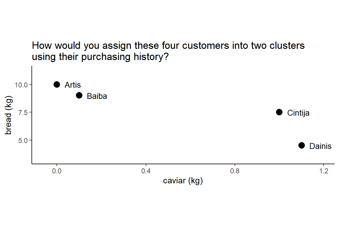
Ready?
Did you assign Artis with Baiba into one cluster and Cintija with Dainis into another? That’s not what k-means would do without standardizing the variables.
Original variables
Let’s check by performing k-means with \(k=2\).
# Data for clustering.
groceries_num <- groceries_df[-1]
# Reproducibility.
set.seed(1)
# K-means with original variables.
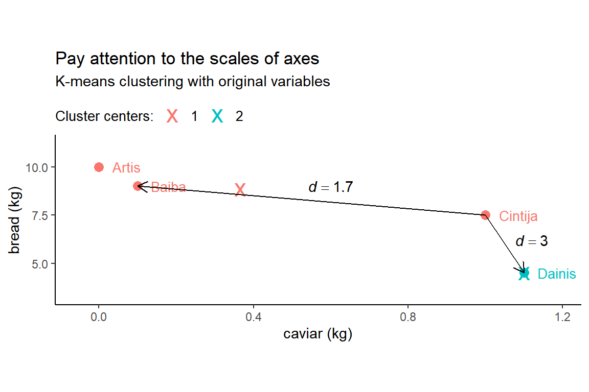
kmeans_orig <- kmeans(groceries_num, centers = 2)The result is plotted below with Dainis being alone in cluster 2 and all other customers in cluster 1. Hopefully, you are surprised.
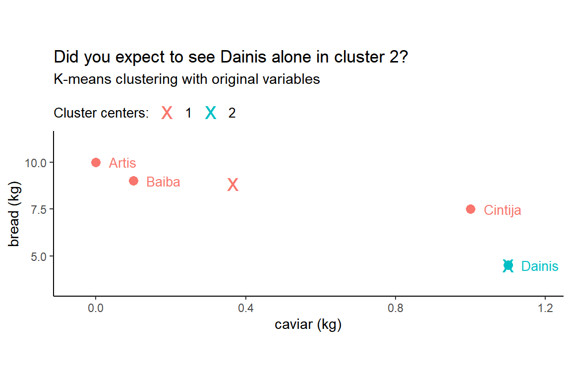
The catch is in the visualization - notice that x and y axes have different scales. The length of one unit on the x axis (i.e. 1 kilo of caviar) is exactly 20 times longer than the length of one unit on the y axis (i.e. 1 kilo of bread). As a result, diagonal distances are hard to evaluate visually. It seems that Cintija is closer to Dainis than to Baiba. But it’s an illusion. Note the distances on the plot below:
All pairwise Euclidean distances can be calculated with dist():
# Add rownames to see customer names in a distance matrix.
groceries_num <- as.data.frame(groceries_num)
rownames(groceries_num) <- groceries_df$customer
# Euclidean distances in kilos.
round(dist(groceries_num), 1)
## Artis Baiba Cintija
## Baiba 1.0
## Cintija 2.7 1.7
## Dainis 5.6 4.6 3.0If we re-plot the same data set while ensuring that one unit on the x-axis (i.e. 1 kilo of caviar) has the same length as one unit on the y-axis (i.e. 1 kilo of bread), the k-means result is no longer a surprise:
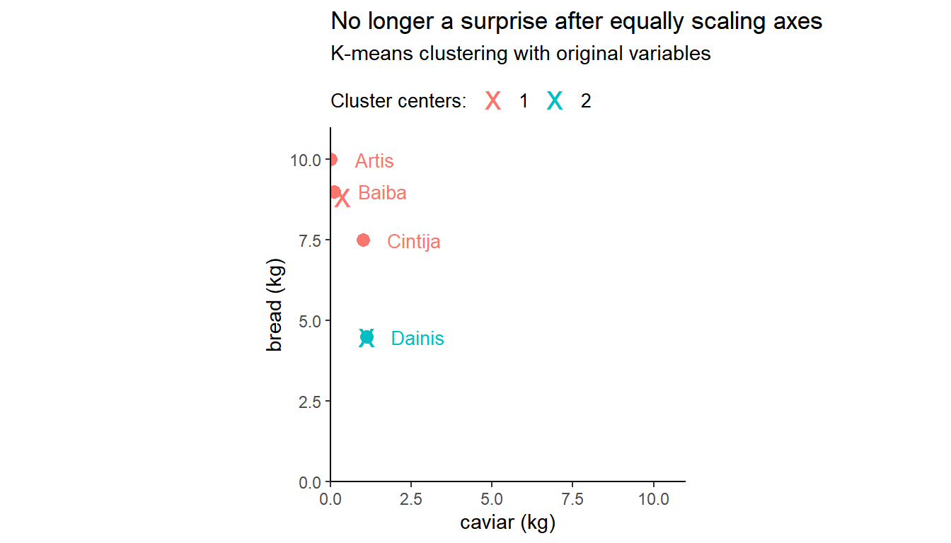
Now this clustering may look correct as Dainis stands away from other customers. However, acknowledge that caviar is a delicacy. In comparison with bread, it is consumed in considerably smaller amounts and it is priced considerably higher. Therefore, a difference of 1 kilo of caviar in customer purchasing habits is more important than a difference of the same weight of bread. A calculation of distances using original, or non-standardized, variables does not differentiate between caviar and bread, essentially assuming these two products are identical. To summarize, a higher variation in bread weights makes this product be more important for Euclidean distance calculations and, as a result, for clustering results.
So the results of clustering depend on the variation of variables in the data set. We can resolve this problem by standardizing the data prior to the clustering.
Standardized variables
Different standardization methods are available, including z-standardization (also called z-score standardization) and range standardization. Z-standardization rescales each variable \(X\) by subtracting its mean \(\bar{x}\) and dividing by its standard deviation \(s\):
\[Z=\frac{X-\bar{x}}{s}.\]
After z-standardization each variable has a mean \(\bar{z}\) of 0 and a standard deviation \(s\) of 1. Z-standardization can be done with scale().
In cluster analysis, however, range standardization (e.g., to a range of 0 to 1) typically works better (Milligan and Cooper 1988). Range standardization requires subtracting the minimum value and then dividing it by the range (i.e., the difference between the maximum and minimum value):
\[R = \frac{X - X_{min}}{X_{max} - X_{min}}\]
We can write a one-line function to perform range standardization:
standardize_range <- function(x) {(x - min(x)) / (max(x) - min(x))}Then apply our new function to each column:
groceries_num_scaled <- apply(groceries_num,
                              MARGIN = 2,
                              FUN = standardize_range)
groceries_num_scaled
## caviar_kg bread_kg
## Artis 0.00000000 1.0000000
## Baiba 0.09090909 0.8181818
## Cintija 0.90909091 0.5454545
## Dainis 1.00000000 0.0000000Notice that each column now has a range of one.
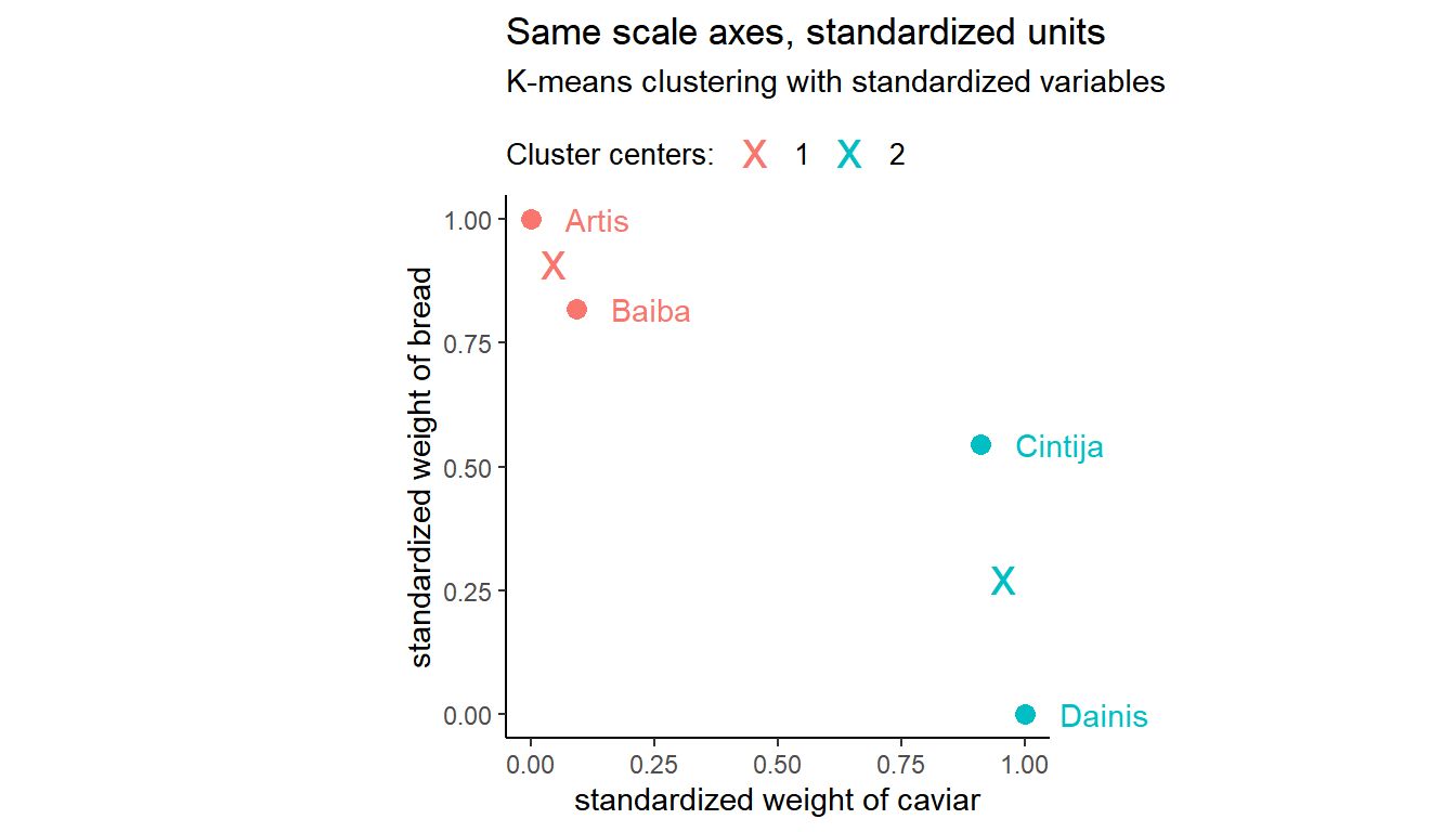
Repeat k-means clustering using standardized variables:
set.seed(1)
kmeans_scaled <- kmeans(groceries_num_scaled, centers = 2)
The results have changed. Artis and Baiba are now in cluster 1 - customers buying 9-10 kilos of bread and almost no caviar. Cintija and Dainis are in cluster 2 - customers buying less bread but loving caviar.
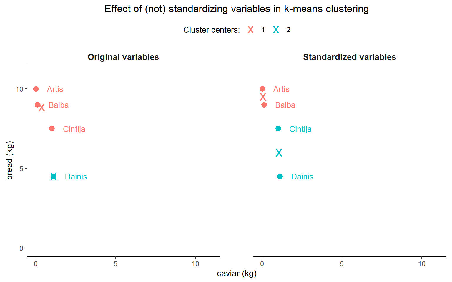
Results
Below is the side-by-side illustration of the effect of variable standardization on k-means clustering. Clustering plotted on the left uses original variables and does not differentiate between a kilo of caviar from a kilo of bread. Clustering plotted on the right uses standardized variables and takes into account the fact that caviar is a delicacy purchased in considerably smaller volumes than bread.
Conclusions
Perform exploratory data analysis prior to clustering and be aware of the differences in variation of variables. Variables with higher variation tend to have a higher impact on clustering. There is no single correct method of standardization. (James et al. 2017, 400) suggest trying several different choices and looking for the one with the most useful or interpretable solution. (Milligan and Cooper 1988) show that the range standardization typically works better for hierarchical clustering, and that z-standardization may even be significantly worse than no standardization in the presence of outliers. If there are outliers, a possible alternative is to use the median absolute deviation instead of the standard deviation (Spector 2011, 160).
I would appreciate any comments or suggestions. Please leave them below, no login required if you check “I’d rather post as a guest.”